22C:21: Computer Science II: Data Structures
Project 3. Posted 11/26. Due 12/13
UNDER CONSTRUCTION
Introduction
This project mainly consists of three, fairly independent parts.
These parts will involve modifying the myWeightedGraph
class.
- Modify the myWeightedGraph class
so that it contains an efficient implementation of Prim's MST Algorithm.
The myWeightedGraph class
should provide the same three functions as before:
	int[] MST()
	myWeightedGraph MSTGraph()
	double costMST()
as before, but as explained in Homework 10,
the algorithm should run efficiently, i.e., in (m + n)*log(n) for arbitrary graphs and
n*log(n) for sparse graphs.
- Currently, the shortestPath method in myWeightedGraph class
returns a shortest path, measured in hops, between a source vertex and a destination vertex.
This method uses breadth-first search to compute shortest paths.
But, now that our graphs are edge-weighted, it makes sense to have two versions
of the shortestPath method, one that measures path length in hops and another
that pays attention to edge-weights.
You will use Dijkstra's shortest path algorithm to compute shortest paths
in an edge-weighted graph.
This algorithm is similar to Prim's MST algorithm.
Details are given below.
- One big source of inefficiency in the graph classes we have implemented thus far
is the getIndex method.
In the current implementation, getIndex simply performs a linear scan of
the names array to find the given vertex name.
This takes linear time (in the worst case) and can become a bottle-neck for other operations
that depend on it.
To fix this problem, I want you to store vertex names in a hash table.
Since we have studied hashing with chaining, you can use that technique and in particular, you
can use the Dictionary class.
Dijkstra's Shortest Path Algorithm
Finding shortest paths in edge-weighted graphs is an extremely common operation - think about the
times you have used MapQuest or Google maps to find shortest
paths.
In addition to its obvious use in online maps, shortest path problems occur in other applications such as
transportation, internet routing, etc.
Dijkstra's shortest path algorithm
(named after Turing award winner, Edsger Dijkstra) is a simple algorithm to compute shortest path
in an edge-weighted graph, with non-negative edge weights. For the rest of this handout, we will assume
that all edge weights in our graphs are non-negative.
Here is the pseudocode for Dijkstra's algorithm - I copied it from Wikipedia and modified it slightly
to match our conventions and language.
This algorithm computes the shortest paths to all vertices in the graph from a given source vertex.
As in the case of breadth-first search, the algorithm constructs and returns a shortest path tree rooted
at the source vertex.
The tree is stored in an int[] called previous that keeps track of the parent of each vertex, in the shortest
path tree.
You should think of Q as a PRIORITY QUEUE ADT;
if you want to be more specific, you can think of it as a min-heap.
The quantity weight(u, v) on Line 11 refers to the weight of the edge {u, v}.
 1  int[] Dijkstra(source)
    {
 2     for each vertex v            	     // Initializations
       {
 3         dist[v] := infinity               // Unknown distance function from s to v
 4         previous[v] := -1		     // the array previous stores parent info.
 5         Q.insert(v)			     // Insert all vertices into the priority queue Q
                                             // The dist-values are used as priorities
       }

 6     dist[source] := 0                     // Distance from source to source is set to 0
 7     Q.change(source, 0)                   // and this is updated in the priority queue as well

 8     while Q is not empty:                 // The main loop
       {
 9         u := Q.delete()                   // Remove best vertex from priority queue; returns source on first iteration
10         for each neighbor v of u:         // where v has not yet been considered
           {
11             alt = dist[u] + weight(u, v)
12             if alt < dist[v]              // Relax (u,v)
               {
13                 dist[v] := alt
14                 previous[v] := u
15	           Q.change(v, dist[v])
	       }
	   } // end of for-each-neighbor
       } // end of while-Q-is-not-empty
16     return previous[]
    } // end of function
Dijkstra's algorithm starts by assigning a "distance estimate" to each vertex. These are stored in the array
dist.
As the algorithm proceeds the distance estimates will improve and eventually reach the correct values.
Initially dist[source] is set to 0, whereas all other distance estimates are set to infinity, reflecting
the fact that the distance from source to itself is obviously 0 and the fact that the other vertices are yet
to be reached.
The correctness of Dijkstra's algorithm relies of the following fact (which will be proved in the Algorithms
course, 22C:21): the vertex in Q with smallest distance estimate, has the correct distance estimate.
This allows us to perform the delete operation on Q and extract the vertex u,
with smallest distance estimate (Line 9).
At this point, vertex u is considered settled; it will never reenter Q.
Then we visit each neighbor v of u to check if dist[v] can be improved by traveling
to v via an alternate path that involves going from source to u along a shortest path
and then taking edge {u, v}.
If this alternate shortest path is an improvement, then dist[v] is improved (Lines 12-15) and the
heap is updated to reflect the change in the priority of vertex v.
It is easy to see that the main loop in the code runs n times, picking out one vertex
from Q in each iteration.
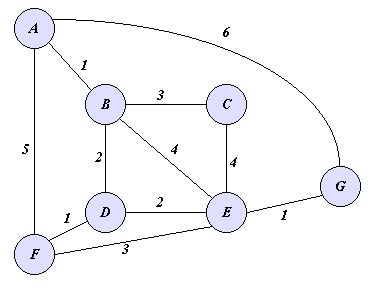
As an illustration, consider the edge-weighted graph shown below and suppose
that we want to compute shortest paths from vertex A to all other vertices
in the graph.
 Then initially the heap will contain all vertices, with A having priority
0 and the remaining vertices having priority infinity.
The following table shows the execution of Dijkstra's Shortest Path
algorithm; each row corresponds to the state of the algorithm before
each iteration. The first row describes the initial state of the algorithm.
The entry "I" stands for infinity, the entry "S" stands for "settled"
(i.e., a vertex which has exited the heap); any vertex that is not
"S" corresponds to the priority of that vertex in the heap. So, for example,
Row 3 tells us that before iteration 3, Q contains vertices C, D, E, F, G
with priorities 4, 3, 5, 5, 6. Since D has lowest priority, it exits Q
in iteration 3.
The one "interesting" event that happens during the execution of this
algorithm, happens in iteration 3, during which a path A-B-D-F of length
4 from A to F is discovered.
Note that even though this path is 3 hops long it is shorter than the
1-hop path A-F.
A 	B 	C 	D 	E 	F 	G
0 	I	I	I	I	I	I
S	1	I	I	I	5	6
S	S	4	3	5	5	6
S	S	4	S	5	4	6
S	S	S	S	5	4	6
S	S	S	S	5	S	6
S	S	S	S	S	S	6
S	S	S	S	S	S	S
Based on the above description, implement the following methods as part of the myWeightedGraph class.
- int[] DSP(String source): As described in Homework 11, this method
reurns the shortest paths from the vertex source to all other vertices, stored as a tree rooted at
source.
- String[] shortestPath(String source, String dest, String attribute): The argument attribute
can take on two valid values: "hops" and "weights."
When the value of attribute takes on the value "hops," the method should return a shortest path in hops
from the vertex source to the vertex dest.
This we have already computed by using the breadth first method.
When the value of attribute takes on the value "weights," the method should return a shortest path, that takes edge weights into consideration,
from the vertex source to the vertex dest.
This is computed by calling the method DSP.
Feel free to add other methods that provide other information about shortest paths.
Using a Hash Table to Store Vertex Names
The getIndex method in our graph class is a big bottleneck;
as implemented it takes linear time (in the number of vertices) and gets
called very often from the other methods in the class.
One way to fix this problem is to use a hash table (see for example, the
Dictionary class) to store vertex names.
One way to do this is to define a Vertex object that keeps
track of (i) the name of the vertex and (ii) the neighbors of the vertex and
store Vertex objects in the hash table.
More specifically, each Vertex object should have (at the very
least) the following fields:
- A String field that stores the name of the vertex.
- An EdgeLinkList field that stored the list of neighbors
of the vertex, along with weights of edges connecting the vertex
to neighbors.
The String field (i.e., the name of the vertex) will be used to
hash each vertex into a slot in the hash table.
Collisions are deal with (as before) using chaining.
Thus the hash table will be an array of linked lists of Vertex
objects.
Making this change has a pretty significant impact on the graph class.
Here are some of the implications.
- There is no longer an implicit correspondence between vertex names
and indices.
There are many method in the graph class whose arguments are vertex indices;
you can get rid of all of these.
- There is no getIndex method any more. Instead, there is
search method that takes a vertex name, searches the hash table
for it, and returns the Vertex object corresponding to that
vertex name.
For example, the code for the method addEdge might look like:
	public void addEdge(String vertex1, String vertex2, double w)
	{
		// Here names is the Dictionary object (i.e., hash table)
		// that needs to be searched. search returns a valid
		// Vertex object or null
		Vertex i = names.search(vertex1);
		if(i == null)
		{
			System.out.print("addEdge failed: ");
			System.out.print(vertex1);
			System.out.println(" does not exist.");
            		return;
        	}

		Vertex j = names.search(vertex2);
		if(j == null)
		{
			System.out.print("addEdge failed: ");
			System.out.print(vertex2);
			System.out.println(" does not exist.");
            		return;
        	}

		// Recall that each Vertex object has field for
		// vertex names and a field for neighbors of that vertex.
		// As usual neighbors can just be an EdgeLinkList
		// Then something like the following will work

		i.neighbors.insertFirst(vertex2, w);
		j.neighbors.insertFirst(vertex1, w);

	}
- You might want to make the load factor of the hash table about
1/5 by choosing a hash table size to be a prime number
about 5 times the number of vertices that the table is supposed to hold.
Remember that the user may or may not specify (in the graph constructor
call) how large their graph might be.
If the user provides no information, assume (somewhat arbitrarily) that
the graph will have about 1000 vertices; otherwise, use the number
provided by the user.
Also make sure that the resize method still works. Earlier
we had two resize methods, one for the names array and one for the Edges
array; now you just need one.
When you resize and use a larger array you need to make sure that all
the items in the old array are rehashed into the new array.
This is because the hash function changes as the size of the array changes.
This part of the project is different from the other parts because it
involves making a lot of minor changes to various parts of the graph class.
Therefore, it is easier to make mistakes/typos etc.
My suggestion is to comment out most of the graph class and one-by-one
uncomment, modify, and test each method.
You should not move on to the next method until the method is completely
tested.
Experiments
You should have two graph classes: one called myWeightedGraph
and the other called myWeightedFastGraph.
The myWeightedGraph is the graph class before you made
the transition to using a hash table for the vertices.
It should contain all the graph methods we have discussed including
methods related to Dijkstra's shortest path (mentioned above in this
handout).
The myWeightedFastGraph class is what you get by modifying
the myWeightedGraph class so that vertices are stored in
a hash table.
It is ok for the myWeightedFastGraph class to be incomplete
in the sense that it may not contain all of the methods of the
myWeightedGraph class. But, it is important that whatever
it contains be correct and well-tested.
Perform the following experiments.
- By performing Experiment 1 in Project 1 we discovered that
it is not possible to travel from Yakima, WA to Wilmington,
DE along edges of length at most 200 miles. However, if we use edges of length
at most 450 miles then yes, this is possible (see my
output for Project 1).
Find a shortest path in miles from Yakima, WA to Wilmington, DE in
the city graph containing all 128 cities and edges of length at most 450 miles.
You will be using the shortestPath method with
attribute "weights."
It is fine to use the myWeightedGraph class for this experiment.
-
As in Homework 10 and
Homework 11, generate 20 random graphs, each
with 10,000
vertices and a probability of 30/9999 of each pair of vertices being
connected by an edge.
To each vertex assign a random String as a name
(see generating a random string to see how to do this).
Perform this task using the myWeightedGraph class as well
as the myWeightedFastGraph class.
Output the time it takes to build the graphs using each of the two classes.
Comment on how much longer it takes to build the graph using the
myWeightedGraph class.
-
Even though an MST and a shortest path tree are computed using similar
algorithms (Prim's and Dijkstra's), they can be quite different from each
other. An MST minimizes the total weight/cost of the tree whereas a
shortest path tree minimizes the weight/cost of each path from a
particular source vertex.
To investigate this difference generate 10 random graphs with edge
probability 0.5.
Assign random real weights in the range [1, 100] to the edges.
For each graph compute an MST (call it M) and then compute a
shortest path tree (call P) from an arbitrarily chosen vertex (call it s).
Report the total weight of M and P - you should see that P's weight
is at least as much as M's weight.
Also report the the average distance from all vertices to s in M as well
as in P - you should see that the average distance in M is at least
as much as the average distance in P.
Note that you will be reporting 4 numbers for each generated graph and
therefore a total of 40 numbers.
It is fine to use the myWeightedGraph class for this experiment.
Explain the plots your results.
-
Ignoring the TSP methods, the costliest methods in the graph
classes are probably
connectedComponents, MST, and DSP.
In this experiment you are asked to compare the running times of these
methods in myWeightedGraph class to the running times in
myWeightedFastGraph class.
Generate random graphs for n = 10000, 10100, 10200, 10300,..., 10900 with
p = 30/(n-1); assign a random real weight in [1, 100] to each edge and
assign a random string name to each vertex.
For each of the 10 (n, p) values mentioned above, generate 10 random graphs
with that value of n and p.
Make sure that each generated graph is also connected up,
in the way described in Homework 10
and has just one connected component.
Compute the MST of each graph and then run DSP to compute
shortest paths from an arbitrarily chosen source.
Do this once with myWeightedGraph and once with
myWeightedFastGraph.
Report separately for each implementation (i) the average time it took to check if the graph is
connected or not, (ii) the average time to compute an MST, and (iii) the
average time it took to run DSP.
These averages are computed over the 10 runs with the same value of n.
Make 3 plots, one for connectedComponents, one for
MST, and one for TSP. Each plot should show the running
time of the method in myWeightedGraph and in
myWeightedFastGraph as a function of n.
Explain the plots you get.
What to submit
Submit all you source code in a zip file.
Submit a "README" file - call it project3.readme, that enumerates
errors, incomplete implementations, extremely slow methods, etc.
You'll loose extra points if we find errors not listed in
your "README" file, so it is important for you to have a good sense of
how correct your implementation is.
Submit a file called project3.pdf that contains the output
of your experiments, the plots, and your explanation of the plots.

