An Epidemic Simulator
by
Douglas W. Jones
|
This epidemic simulator allows the progress on an epidemic to be tracked through a community, where people in the community perform various roles that involve visits to places where contageous people can spread the disease.
In each simulated person, the disease progresses from latent (non-infectious) through asymptomatic, symptomatic, and bedridden states to either recovered (non-infectious and immune) or dead (also non-infectious). Places are characterized by their "transmissivity," a parameter that determines the likelihood that a person occupying that place will become infected (as a function of the number of infectious people there and the duration of stay).
The effectiveness of mitigation strategies can be measured comparing outcomes with the transmissivity of places adjusted to model the effect of social distancing or mask wearing requirements. Screening policies can be attached to places to exclude contageous people and recommend that they self-quarantine. People in different roles can be given different levels of quarantine compliance, and the effect of closing certain categories of places can be modeled by comparing model runs with and without those places.
Multiple runs of the model tend to produce different results because of the randomization of which simulated people get infected when visiting a place, randomization of who is initially infected, randomization of the roles assigned to different simulated people, and random choices the people in some roles make to visit or not visit certain places. As a result, it is practical to make multiple simulation runs to explore the spread of outcomes that could result from some initial state.
The underlying simulation mechanism uses discrete-event simulation, tracking the movements of individual simulated people. As such, this simulator can easily handle a few thousand people but is unlikely to be useful for populations in the millions.
| Resist Russian Imperialism | ||
Input to the simulator is given in a text file that describes the disease and the community. Here is an example:
population 100;                     latent       2.0 day 0sec;
infected 1;                         asymptomatic 2   day 0;
place home  10  0 0.01;             symptomatic  2       0   90%;
place work  10  0 0.01;             bedridden    2       0   90%;
role homebody 60 home;
role worker   40 home work (9:00AM-5:00PM);
end 30 days;
This file contains the following elements:
First, there is a specification of the population, 100 people of which just one is initially infected.
population 100; # total number of people
infected 1;     # of them, how many are initially infected
Second, there is a description of the disease. This rather unrealistic disease takes exactly 2 days to progress from disease state to disease state. 90% of those in the symptomatic state will recover without becoming bedridden, and 90% of those in the bedridden state will recover. The remainder will die.
# stages of the infection
latent       2.0 day 0sec;
asymptomatic 2   day 0;
symptomatic  2       0  90%;
bedridden    2       0  90%;
Third, there is a description of the places in this community. This community consists of homes and workplaces, each with a capacity of 10 plus or minus 0 people. Both homes and workplaces have an transmissivity of 0.01, meaning that if there are c contageous occupants in one of these places the expected time until infection for a newly arrived person is 1/0.01c or 100/c hours, where the actual time will be drawn from an exponential distribution. For low transmissivities, a seat-of-the pants interpretation of a transmissivity of 0.01 is that if a person shares a room with one contageous pereson for one hour, they have about a 0.01 probability of infection.
# the categories of places in this community
place home  10  0 0.01;
place work  10  0 0.01;
Fourth, there is a description of the population of this community and how they relate to the places. Here, 60% of the population is made up of homebodies who just stay home, while 40% of the population is made up of workers who start from home and go to work from 9:00 AM to 5:00 PM daily, potentially spreading the disease from home to home.
# people and their relationship to places
role homebody 60 home;
role worker   40 home work (9:00AM-5:00PM);
Finally, there is a specification of how long the simulation is to run. This example runs for 30 simulated days.
end 30 days;
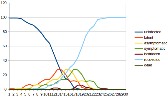
The output of this simulator is in CSV format. Free tools such as gnuplot can be used to convert such output to high quality graphs. Here is the output of one run of the simulator with the above input, as graphed by LibreOffice Calc, a free and widely available spreadsheet program. The data was plotted using the line graph option without data points and using the default axes, default title and default scale settings:
|
|
Each component of the model specifiction begins with a keyword, followed by various fields, followed by a semicolon. Fields may be separated by whitespace (spaces, tabs and newlines). The components of the model specification may be given in any order, except as noted. In the following description, square braces are used to surround optional fields, curly braces surround fields that may be repeated. The components are:
Each place category must have a distinct name so that roles can refer to the places visited by the associated people. Actual places in that category are created, as needed, to accomodate the people associated with that place.
Transmissivities are given in infections per hour per contageous person sharing that place. Given that the transmissivity of a place is p and c contageous occupants, the expected time in hours until infection for an uninfected occupant is 1/pc and the actual time will be drawn from an exponential distribution with this mean.
Places have optional screening rules. If a place has a screening rule, those entering the place are subject to screening; those deemed infectious are sent home. Screening rules are specified as follows:
The total population is divided between roles proportionally to the fractions of people declared for each role. This proportional division allows the fraction to be given as a percentage or an absolute number of people, so long as the numbers are used consistently for all roles in the model.
The compliance probability gives the likelihood that a person in this role who has been told to self-quarantine after screening at some place will comply with that order. 1.0 or 100% implies fully compliant.
The list of places must include at least one place. Each place named must correspond to a place that has already been specified.
Exactly one place must be given without an associated schedule; each simulated person in this role will be assigned a home constructed from that category of place. The schedules given for other places describe when and if a person in this role will travel from their home to a place in the indicated category.
No place may be mentioned more than once in conjunction with any role. Schedules for the places mentioned in any role must not overlap.
The total number of people associated with any kind of place will be distributed among the places of that kind randomly.
Schedules are written as:
The optional specification of what days gives the days on which the schedule applies to people in this role. If the days are not given, the schedule applies daily, as modified by the probability and illness.
The optional probability gives the probability that any particular person will follow this schedule on any particular day. The probability defaults to 1.0, meaning 100%, in which case, the schedule is always followed (except when the person is bedridden).
The fields mentioned above have the following formats:
All numbers for fields of times are given in <float> format, so all of the following times are approximately equivalent: 10:34:15pm, 10:34.25pm, 10.57083pm, 22:34:15 and 22.57083.
Spaces around elements of a time are optional,
so 1 hr AM means the same as 1hrAM
and 1 : 00 am means the same as 1:00am.
Where a <day range> is <day> { - <day> }
Where a <day> may be:
Spaces may be inserted or omitted before and after punctuation, so
Mon-Thu is the same as Mon - Thu.
Also note that the order of the days in a range matters.
Mon-Thu means Mon,Tue,Wed,Thu while
Thu-Mon means Thu,Fri,Sat,Son,Mon.
The number specifying the probability is given in
<float> format.
Spaces between the number, optional percent sign, and what follows are optional,
so 1 % means the same as 1.0%.
Comments begin with a pound sign (#) and continue to the end of line. Comments are allowed in most places, but most comments will be either full-line comments between sections of the model specification or comments at the end of line after semicolons or between the place names of a role.
The simulator output is in CSV format, that is, Comma-Separated Value format. This is a common ad-hoc data format used by many spreadsheet, database and graphing tools. The first line of the output file is a headline, while the following lines give the corresponding data for each daily report. The simulation always starts at midnight and daily reports are made at midnight. Here are the first few lines of the output that was used to produce the graph given above.
time,uninfected,latent,asymptomatic,symptomatic,bedridden,recovered,dead
0.0,99,1,0,0,0,0,0
1.0,99,1,0,0,0,0,0
2.0,99,0,1,0,0,0,0
3.0,98,1,1,0,0,0,0
4.0,94,5,1,0,0,0,0
5.0,91,7,1,1,0,0,0
6.0,89,5,5,0,0,1,0
7.0,84,7,7,1,0,1,0
By the end of the 7th day, the person who was initially infected has recovered from the disease, but in that time, 15 more people have been infected, 8 of whom are infectious and one of whom is symptomatic.
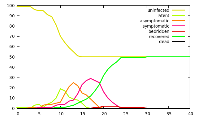
Here is an example that is interesting because there are two communities, call them martians and earthlings, that are only loosely linked because just a tenth of the community visits a third place, call it the moon, for an hour daily. While on the moon, simulated people take care to cut their probability of infection way down. The net result is that it is quite possible for one planet to entirely escape the epidemic while it is also quite possible for the epidemic to jump between planets. The disease described here is somewhat more realistic than the one described in the first example because there is a random element in the duration of some of the disease stages.
population 100;                     latent       2.0 0;
infected 1;                         asymptomatic 3   0;
place earth 100 0 0.001;            symptomatic  5   24hr 0.9;
place moon  100 0 .0001;            bedridden    8   48hr 0.9;
place mars  100 0 0.001;
role human   .5 earth  moon (11 am -noon  10%);
role martian .5 mars   moon (11    -12    10%);
end 30;
Here is the output of a run with the above model where, by sheer luck, the epidemic did not jump between the two planets. This plot was made using gnuplot, overriding the default colors and line thickness but otherwise leaving it to decide the layout of the plot. The simulation output does not tell which planet escaped infection because the two have identical populations.
|
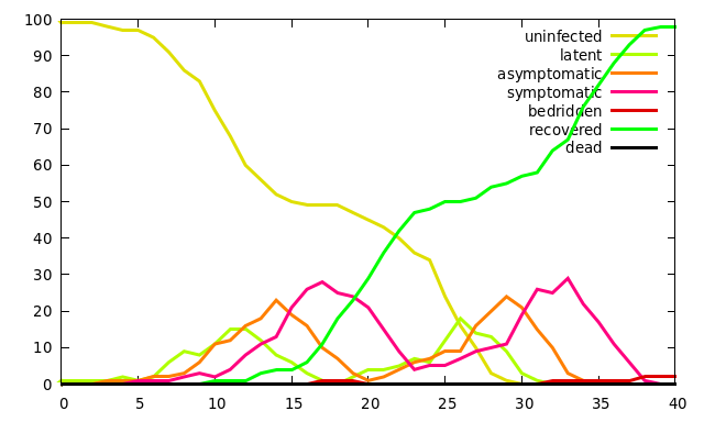
Here is the output of another run with the above model where, with worse luck, the epidemic jumped between the two planets, probably between days 10 and 15, although the output does not tell us exactly when:
|
The onset of the disease in both runs is fairly slow. When the model starts with just one infected person and relatively low transmissivity, there is significant variation in how long it takes for the disease to catch on. Once the number of infected people begins to grow, things are more predictable. Note also that the second output shows two peaks in each disease stage, one peak due to infections on the first planet, and a second peak as the disease sweeps through the second half of the population.
The Epidemic simulator models the propagation of a disease through a community by modeling contacts between people who happen to be in the same place at the same time. To do this, it must create a population and a set of places, and then move people in that population from place to place.
The input language of the simulator works with people collectively by allowing the declaration of any number of distinct roles, where each role makes up some fraction of the population. Each person in each role is associated with a specific list of places that person visits according to that person's travel schedule.
Places are also declared collectively. Place names in the input language refer to categories of places. A category of place will have no instances, when no role is associated with that category of place. There may be only one instance, if the size of the place is large enough to accomodate all of the people associated with that place. The earth-moon-mars example has just one instance of each place.
Usually, there will be multiple instances of each place. Consider this little example:
population 1000;
place home       4   3  0.001;
place classroom 25  10  .0001;
role student 1  home   classroom (8:30AM-3:00PM)
This creates 1000 students and distributes them to on the order of 250 homes. The median home size is 4, and the spread is 3, so most homes will hold between 1 and 7 occupants, using a log-normal distribution. It also distributes the same students between on the order of 40 classrooms. The median classroom size is 25, and the spread is 10, so most classrooms will hold between 15 and 35 students, also using a log-normal distribution.
Homes are created, as needed, to accommodate people associated with them, and classrooms are created similarly. The simulator distributes people to places using a uniform random distribution. As a consequence, each run of the simulator will, with astronomically high likelihood, create a different social network. For the above example, there will be no correlation between student's homes and classrooms. Each of the four or so students living in any particular home has an equal likelihood of being assigned to any of the 40 or so clasrooms, so there is ony about a 1 in 10 chance that two students who share a home will also share a classroom.
The rules for associating people with places do not depend on which place is the person's home place nor do they depend on travel schedules.
The simulator contains no way to force correlated roles with places. Consider this fragment of a model:
place home       4   3  0.001;
place work      10   8  0.001;
place classroom 25  10  .0001;
role student 25 home   classroom (8:30AM-3:00PM)
role teacher 1  home   classroom (8:00AM-5:00PM)
role parent  24 home   work      (8:00AM-5:00PM)
This creates a 1:1 ratio between adults and children, and it creates a 25:1 ratio between students and teachers, but it does not guarantee that there will be one teacher per classroom, nor does it guarantee that every household contains an adult.
The simulator provides no way to vary schedules aside from the pattern of days on which the schedule applies and the random probability that a person will or will not visit a place on any particular day. In the real world, some people arrive late or depart early.
The simulator provides no way for a person to go back to a place. Each person is constrained to visit each scheduled place other than their home at most once a day. In the real world, people do things like going to lunch or running errands from work.
The simulator provides no support for one-time events like concerts or
political rallies. In the real world, these can become superspreader events.
This happened in Philadelphia in 1918, and it happened with several large
events in 2020.
This simulator models the progress of a disease as sequence of stages, or
disease states. These occur in a fixed sequence unless a person
recovers from one of the infected states:
The duration of each disease state is given by a distinct
log-normal probability distribution, and each
disease state is also characterized by a probability of recovery.
For some diseases, a person could potentially recover from the latent
stage, becoming immune without ever becoming infectious. Recovery from an
asymptomatic infection happens for many diseases. Other diseases frequently
progress to symptomatic or bedridden before recovery. With yet others, such
as Ebola, recovery is vanishingly rare.
This model has sharply delineated disease states.
Real diseases don't work this way. Symptoms can come on
gradually, and fade gradually.
In this model, a person is either infectious, with a disease state between
asymptomatic and bedridden, inclusive, or they are not.
In the real world, infectiousness is not binary.
Rather, an infected person has a degree of infectiousness, shedding
infectious agents at different rates at different times during the
infection and at different rates depending on what they are doing.
In this model, infection is only passed person to person between people
who are in the same place at the same time. In the real world, infection
can be passed by contact. An infected person can deposit infectious agents
on a surface that infect another person several hours later.
In this model, every uninfected person in some place over the same interval
has exactly the same probabilty of catching the disease.
In the real world, individual desicsions such as the decision to wear or not
wear a mask can have a real impact on a person's likelihood of infection.
In this model, recovery from infection always confers permanent immunity.
In the real world, some diseases induce only temporary immunity that fades
with time.
In this model, all people are strictly equal with regard to the disease,
except that those who have recovered are totally immune. In real life,
differences in age or preexisting conditions have a serious impact on the
outcome of an infection. The 1918 flu epidemic hit young people harder.
The 2020 COVID-19 epidemic hit older people harder.
This simulator draws random numbers with three distinct probability
distributions. Uniform distributions are used to spread people over places,
exponential distributions are used to determine the time until infection in
a place, or equivalently, the likelihood a person will be infected after
a particular time in a place, and log-normal distributions are used for
the distributions of place sizes and disease state durations.
When distributing initial infections over the set of all simulated people,
each simulated person has exactly the same likelihood of being infected.
If n people are to be infected, the algorithm used is equivalent to
drawing n people from the population at random and infecting them,
with no regard to each person's role or place.
When assigning people to places, people with an association with some category
of places are drawn in random order and spilled into places, creating new
places from that category as needed until all of the people are emplaced.
The net result does not guarantee that every place is filled
to capacity because this approach usually generates excess
capacity. Imagine, for example, places with a capacity of exactly 10
people being created to meet the demands of a population of 100. This
implies the creation of a total of 10 places, with an aggregate capacity
of 100 people.
The probability that a person will become infected when in some place
depends on the number of contageous people there, the duration of stay and
a property of that place, its transmissivity. Transmissivity may
be seen as parameter that aggregates all of the properties of the place that
have an impact on infection, from the quality of the ventilation through
the use of ultraviolet light to the social distancing and mask wearing
policies of the place.
For small probabilities of infection, doubling the duration of stay doubles
the likelihood of infection and doubling the number of contageous people in the
place doubles the likelihood. This suggests that, near zero, the infection
probability is approximately linear with the number of contageous people and
the duration of stay.
Consider a person who has spent some time in a room but is still uninfected.
If that person steps out of the room for even an infinitesimal time and
then steps back in, their previous history in the room is irrelevant and their
probability of infection can be computed in terms of their recent entry to the
room. There is only one probability distribution that works like this, the
exponential
distribution.
The mathematics of radioactive decay works identically to the mathematics of
infection, so we can speak of the halflife of a decay process as being
analogous to the time until half the formerly uninfected people in a room
are infected by the contageous people in that room.
There are two ways of looking at the probabilities here:
First, the probability of a person being infected after a time t as
a function of the number of contgeous people in the place c and the
transmissivity of the place p is:
P(infection before time t)
= 1 – e–pct
When the product pct is small, this is approximated by:
P(infection before time t) = pct
This conforms to our intution that doubling the number of contageous people in
a place c, doubling the transmissivity of that place p
or doubling the time t spent in a place should all double the
probability of infection.
Alternatively, we can speak of drawing a random time when a person enters
a place that determines when that person will become infected, as a function of
the number of contgeous people in the place c and the
transmissivity of the place p. Where the formulas given above are
for the cumulative distribution function, now, we want the probability
distribution function for the same distribution:
P(t)
= pc e–pct
The mean value of this distribution is 1/pc and the median
is (ln 2)/pc. The latter allows us to translate
epidemiological data to the transmissivity of a place because the
median is the halflife. If there are a large number of people in
the place, in addition to c contageous people,
we expect half of the previously uninfected people will
become infected by time
t = (ln 2)/pc
Therefore, if you measure the time thalf
until half the people are infected,
you can compute the transmissivity of the place as
p = (ln 2)/cthalf
≊ 0.69/cthalf
Demographic distributions such as the number of
occupants in a household, or the number of students per school can be easily
approximated by discretized log-normal distributions, so we use a log-normal
distribution to describe the distribution from which the populations of
places are drawn when distributing simulated people to each category of place.
It is somewhat more difficult to find detailed data on the durations of
different stages in the progress of a disease, in part because the time of
initial infection is frequently unknown, and in part because many people recover
from asymptomatic (but contageous) diseases without contributing to our
statistics for those diseases. Nonethess, we speculate that a log-normal
distribution might be a useful approximation for the duration of a disease
stage because it allows for a long tail of those for whom the disease stage
lingers while allowing the bulk of those who are infected to recover in a
relatively short time.
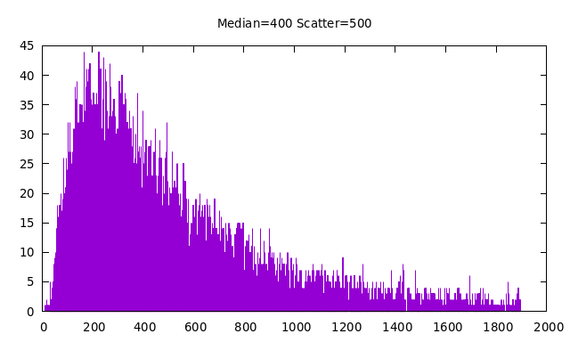
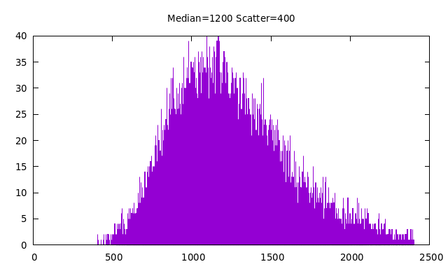
The log-normal distribution is typically described by two parameters, the
median value and σ, the standard deviation of the logarithm of the random
value. Working with sigma is not intuitive, so here, we use a more natural
set of parameters:
m -- the median of the distribution
s -- the scatter of the distribution
Formally,
σ = ln( (s + m) / m )
This allows descriptions to be given intuitively because most of the mass of
the probability distribution will be between
m–s and m+s.
You can see this in the following examples:
The Disease Model
Simulated people remain in this state until they are infected, either
when the simulation model is initialized, or by contageon from a
contageous person in some shared place.
Upon infection, the disease is latent, which is to say, neither
exhibiting symptoms nor contageous.
After a random interval, the person becomes contageous, but does
not know it because there are no symptoms.
After a random interval, the person becomes symptomatic; they know
they are sick and probably contageous, but continue about their normal
activities, "toughing it out."
After a random interval, the person becomes bedridden; they are so
sick that they stay home. They may still infect those they share a home
with.
After a random interval, the person dies. They are removed from the
model and no longer pose a threat of contageon.
The person is no longer contageous and is permanently immune from further
infection.
Limitations
Probability Distributions
Uniform Distributions
Exponential Distributions
Log-Normal Distributions
|
|
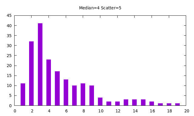
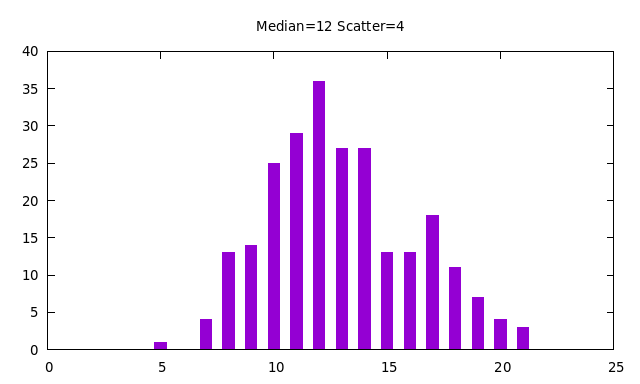
Household sizes and school enrollments never involve fractonal people, so when numbers are drawn from a log-normal distribution for such purposes, they must be converted to integers. We do this by rounding up all fractional values to the next integer. The probability of 0.0 under the log-normal distribution is exactly 0, so rounding up gives a minimum value of one. You can see this in the following examples based on the previous two examples:
|
|
The software used to produce all of the above plots is here. It is not difficult to use this software to make "eyeball fits" to published probabilty distributions for various demographics. In a bit more detail, the above plots are histograms of the results of a number of trial draws from the distribution, using bins from zero to 3 times the scatter above the median. The number of trials is always 10 times the number of bins.
Support for screening policies is a bit rudimentary The time taken by screening is not explicit. It ought to be given, since antigen screening, in particular, can be time consuming and there is rapid progress being made on new and faster tests, with an interesting tradeoff between speed and accuracy.
It would be interesting to add "jitter" to schedules, so that all the people in a role didn't all select the same time to go to each scheduled place. Employers want their employees to all arrive on time, but restaruants really prefer their customer arrivals to be scattered throughout their open hours.
It would also be possible to add commute times. As the simulator currently works, commuting is instantaneous. It would be somewhat difficult to make people carpool, but fairly easy to add to each place a specification of the average travel time to that place and the variation, assuming that each traveler travels independently, as if they all had single-occupancy cars.
The current veresion of this epidemic simulator is available here. This distribution of the code is released as free software under the General Public License (GPLv3). See the README file for details.
The simulator is a modestly large Java program, over 2000 lines of code divided between 14 source files. This code makes extensive use of λ expressions, a relatively recent addition to Java. As a result, this code requires use of Java SE 8 or later.
The simulator is written so that the Javadoc utility may be run over it to produce a web site of internal documentation. As a result, developers will find it useful to keep a web browser open on screen to read documentation for parts of the program while working on other parts of the program.
In addition to the documentation generated from comments in the source code by Javadoc, there is a makefile. This works with the make utility to compile the program, but it also provides a valuable roadmap to the top-level organization of the code, showing which parts of the Java program depend on which other parts, and documenting how the entire collection of code can be viewed as a set of distinct software layers. Finally, the makefile is useful as a script for running the code. Don't type commands to run the program and then more commands to plot the output, just type make plot, adding the name of the model description file to be used as simulator input.
As mentioned above, the simulator produces output in CSV format. Many different utilities can plot graphs from this output, but the scripts embedded in the makefile uses gnuplot, a widely available free plotting utility.
This program is built on a discrete-event simulation framework. That means that time does not advance in fixed size increments, but rather, time jumps forward from event to event, where events are instants in time when some state variable in the model changes. In this simulator, events represent such things as:
Simulating an event may involve such things as drawing random numbers to determine what happens, changing one or more variables representing the state of the model, and scheduling future events that are consequences of this event. When a person becomes contageous, for example, one consequence is scheduling new future events for every person in the same place giving their times of infection. When the last infectious person leaves a place, one consequence will be the cancellation of the infection events for every person still in that place who is not yet infected.
The term agent-based simulation is sometimes used to describe such models, but that term is frequently taken to imply that agents are rational, or that they learn, or that they have some degree of intelligence. The simulated people in this model are not rational, they do not learn, and they have no intelligence. The term individual-based simulation would be more appropriate, because this model does simulate independent individuals.
One particular chain of events is triggered at the start of time. This chain of events performs the daily report at midnight of the overall progress of the disease, as represented by a census of the numbers of people in each disease state. This daily report does not indicate that time advances in one-day quanta.
A pseudo-random-number generator is used for the random elements of the simulation such as the initial placement of people in places, the drawing of recovery probabilities as a person advances from one disease state to another and the durations of each disease state. There is a second independent source of nondeterminism in the simulator: If two events happen to be scheduled at the same time, there is no guarantee which of the two will be simulated first. The order in which two simultaneous events were scheduled does not determine the outcome; instead, internal details of the underlying pending event set determine this and higher level code in this simulator makes no assumptions about the outcome.
Inside the simulator, time is represented as a double-precision floating-point number. Most of the code is independent of the actual scale of this number. Instead, the code uses time units such as day, hour, and minute as scale factors to convert from human-readable times to internal representations. During early development, the floating point value 1.0 was one second. Later, 1.0 was changed to mean one day. Aside from the definitions of the constants representing time-units, this change required no changes to anywhere in the code.
When event times are computed from time delays drawn from a pseudo-random-number generator, the times are computed to the full precision of the double-precision floating-point computation that goes into computing exponential or log-normal probability distributions. This means that the times of things like the moment of infection or the moment of death are given to preposterous precision. In real life, you cannot state the moment of death to one nanosecond of precision. When measured in nanoseconds, death is a gradual process.
This simulator is the result of the assignments developed for the course CS:2820, Object Oriented Software Development offered by the Computer Science department at the University of Iowa, as offered during the Spring 2021 semester. A cruder epidemic simulator was developed during the fall 2020 semester, motivated by the global COVID-19 pandemic. Previous offerings of the course involved development of other simulators for such things as traffic flow in a highway networks, digital logic, and networks of biological neurons (not to be confused with what are now called neural networks). The discrete-event-simulation framework used here grew from those earlier exercises.
The CS:2820 homework assignments web page contains snapshots of the early development of this simulator in the posted solutions to the machine problems, and the lecture notes for several of the lectures include discussions of top-level design decisions and methodology. Note that support for the following features was discussed during the semester but added after the final assignments in the class were completed:
I would like to thank my students for their many comments, complaints and suggestions as they struggled with my code.